- 개요
- 일반 알고리즘
- 의사 코드
- 그림
- C++ 예제
- Java Example
- Complexity Analysis Of The Insertion Sort Algorithm
- Conclusion
고전적인 예를 통해 삽입 정렬에 대해 자세히 살펴보기.
삽입 정렬은 우리가 손에서 카드를 사용하는 방식으로 볼 수 있는 정렬 기술입니다. 카드를 데크에 삽입하거나 제거하는 방식과 유사한 방식으로 삽입 정렬이 작동합니다.
삽입 정렬 알고리즘 기법은 버블 정렬 및 선택 정렬 기법보다 효율적이지만 다른 기법보다 효율성이 떨어집니다. 퀵소트, 머지정렬처럼요.

개요
삽입정렬 기법에서는 두 번째 요소부터 시작해서 첫 번째 요소와 비교해서 넣는다. 적절한 장소에서. 그런 다음 후속 요소에 대해 이 프로세스를 수행합니다.
각 요소를 이전의 모든 요소와 비교하고 적절한 위치에 요소를 넣거나 삽입합니다. 삽입 정렬 기술은 요소 수가 적은 배열에 더 적합합니다. 또한 연결 목록을 정렬하는 데 유용합니다.
연결 목록에는 다음 요소에 대한 포인터(단일 연결 목록의 경우)와 이전 요소에 대한 포인터(이중 연결 목록의 경우)도 있습니다. ). 따라서 연결된 목록에 대한 삽입 정렬을 구현하는 것이 더 쉬워집니다.
이 자습서에서는 삽입 정렬에 대한 모든 내용을 살펴보겠습니다.
일반 알고리즘
1단계 : K = 1에서 N-1
2단계 에 대해 2~5단계 반복: 온도 = A[K] 설정
3단계 : J = K로 설정– 1
4단계 : temp =A[J]
set A[J + 1] = A[J]
0인 동안 반복>set J = J – 1[내부 루프의 끝]
5단계 : set A[J + 1] = temp
[ end of loop]
Step 6 : exit
따라서 삽입 정렬 기법에서는 첫 번째 요소가 항상 정렬된다고 가정하고 두 번째 요소부터 시작합니다. . 그런 다음 두 번째 요소에서 마지막 요소까지 각 요소를 이전의 모든 요소와 비교하고 해당 요소를 적절한 위치에 배치합니다.
의사 코드
에 대한 의사 코드 삽입 정렬은 다음과 같습니다.
procedure insertionSort(array,N ) array – array to be sorted N- number of elements begin int freePosition int insert_val for i = 1 to N -1 do: insert_val = array[i] freePosition = i //locate free position to insert the element whilefreePosition> 0 and array[freePosition -1] >insert_val do: array [freePosition] = array [freePosition -1] freePosition = freePosition -1 end while //insert the number at free position array [freePosition] = insert_val end for end procedure
위에서 삽입 정렬에 대한 의사 코드를 제공하고 다음 예제에서 이 기술을 설명합니다.
그림
정렬할 배열은 다음과 같습니다.
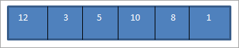
이제 각 패스에 대해 현재 요소를 모든 이전 요소와 비교합니다. 따라서 첫 번째 패스에서는 두 번째 요소부터 시작합니다.
따라서 N개의 요소가 포함된 배열을 완전히 정렬하려면 N개의 패스가 필요합니다.
위 그림을 표 형식으로 요약할 수 있습니다.
| 통과 | 정렬되지 않은 목록 | 비교 | 정렬됨목록 |
|---|---|---|---|
| 1 | {12,3,5,10,8,1} | {12,3} | {3,12,5,10,8,1} |
| 2 | {3,12,5,10,8,1} | {3,12,5} | {3,5,12,10,8,1} |
| 3 | { 3,5,12,10,8,1} | {3,5,12,10} | {3,5,10,12,8,1} |
| 4 | {3,5,10,12,8,1} | {3,5,10,12,8} | {3,5,8,10,12,1} |
| 5 | {3,5,8,10,12,1} | {3,5,8,10,12,1} | {1,3,5,8,10,12} |
| 6 | {} | {} | {1,3,5,8,10,12} |
와 같이 위의 그림에서는 첫 번째 요소가 항상 정렬되어 있다고 가정하므로 두 번째 요소부터 시작합니다. 따라서 두 번째 요소를 첫 번째 요소와 비교하는 것으로 시작하여 두 번째 요소가 첫 번째 요소보다 작으면 위치를 교환합니다.
이 비교 및 교환 프로세스는 두 요소를 적절한 위치에 배치합니다. 다음으로 세 번째 요소를 이전(첫 번째 및 두 번째) 요소와 비교하고 동일한 절차를 수행하여 세 번째 요소를 적절한 위치에 배치합니다.
이러한 방식으로 각 패스에 대해 하나의 요소를 그것의 장소. 첫 번째 패스에서는 두 번째 요소를 그 자리에 배치합니다. 따라서 일반적으로 N개의 요소를 적절한 위치에 배치하려면 N-1 패스가 필요합니다.
다음으로 C++ 언어로 삽입 정렬 기술 구현을 시연합니다.
C++ 예제
#include using namespace std; int main () { int myarray[10] = { 12,4,3,1,15,45,33,21,10,2}; cout"\nInput list is \n"; for(int i=0;i10;i++) { cout ="" Output:
Input list is
12 4 3 1 15 45 33 21 10 2
Sorted list is
1 2 3 4 10 12 15 21 33 45
Next, we will see the Java implementation of the Insertion sort technique.
Java Example
public class Main { public static void main(String[] args) { int[] myarray = {12,4,3,1,15,45,33,21,10,2}; System.out.println("Input list of elements ..."); for(int i=0;i10;i++) { System.out.print(myarray[i] + " "); } for(int k=1; k=0 && temp = myarray[j]) { myarray[j+1] = myarray[j]; j = j-1; } myarray[j+1] = temp; } System.out.println("\nsorted list of elements ..."); for(int i=0;i10;i++) { System.out.print(myarray[i] + " "); } } } Output:
Input list of elements …
12 4 3 1 15 45 33 21 10 2
sorted list of elements …
1 2 3 4 10 12 15 21 33 45
In both the implementations, we can see that we begin sorting from the 2nd element of the array (loop variable j = 1) and repeatedly compare the current element to all its previous elements and then sort the element to place it in its correct position if the current element is not in order with all its previous elements.
Insertion sort works the best and can be completed in fewer passes if the array is partially sorted. But as the list grows bigger, its performance decreases. Another advantage of Insertion sort is that it is a Stable sort which means it maintains the order of equal elements in the list.
Complexity Analysis Of The Insertion Sort Algorithm
From the pseudo code and the illustration above, insertion sort is the efficient algorithm when compared to bubble sort or selection sort. Instead of using for loop and present conditions, it uses a while loop that does not perform any more extra steps when the array is sorted.
However, even if we pass the sorted array to the Insertion sort technique, it will still execute the outer for loop thereby requiring n number of steps to sort an already sorted array. This makes the best time complexity of insertion sort a linear function of N where N is the number of elements in the array.
Thus the various complexities for Insertion sort technique are given below:
Worst case time complexity O(n 2 ) Best case time complexity O(n) Average time complexity O(n 2 ) Space complexity O(1)
In spite of these complexities, we can still conclude that Insertion sort is the most efficient algorithm when compared with the other sorting techniques like Bubble sort and Selection sort.
Conclusion
Insertion sort is the most efficient of all the three techniques discussed so far. Here, we assume that the first element is sorted and then repeatedly compare every element to all its previous elements and then place the current element in its correct position in the array.
In this tutorial, while discussing Insertion sort we have noticed that we compare the elements using an increment of 1 and also they are contiguous. This feature results in requiring more passes to get the sorted list.
In our upcoming tutorial, we will discuss “Shell sort” which is an improvement over the Selection sort.
In shell sort, we introduce a variable known as “increment” or a “gap” using which we divide the list into sublists containing non-contiguous elements that “gap” apart. Shell sort requires fewer passes when compared to Insertion sort and is also faster.
In our future tutorials, we will learn about two sorting techniques, “Quicksort” and “Mergesort” which use “Divide and conquer” strategy for sorting data lists.