- Overview
- Ընդհանուր ալգորիթմ
- Կեղծ կոդ
- Նկարազարդում
- C++ Օրինակ
- Java Example
- Complexity Analysis Of The Insertion Sort Algorithm
- Conclusion
Դասական օրինակներով ներդիրների դասակարգման խորը հայացք:
Մտածման տեսակավորումը տեսակավորման տեխնիկա է, որը կարելի է դիտել այնպես, որ մենք ձեռքի տակ թղթեր ենք խաղում: Ինչպես մենք ցանկացած քարտ տեղադրում ենք տախտակամածի մեջ կամ հեռացնում այն, տեղադրման տեսակավորումն աշխատում է նույն ձևով:
Տեսակավորման ալգորիթմի տեխնիկան ավելի արդյունավետ է, քան Bubble տեսակավորման և Ընտրության տեսակավորման տեխնիկան, բայց ավելի քիչ արդյունավետ է, քան մյուս մեթոդները: ինչպես Quicksort-ը և Merge-ը:

Overview
Ներդիր տեսակավորման տեխնիկայում մենք սկսում ենք երկրորդ տարրից և համեմատում այն առաջին տարրի հետ և դնում այն պատշաճ տեղում: Այնուհետև մենք կատարում ենք այս գործընթացը հաջորդ տարրերի համար:
Մենք համեմատում ենք յուրաքանչյուր տարր իր բոլոր նախորդ տարրերի հետ և դնում կամ տեղադրում տարրը իր ճիշտ դիրքում: Տեղադրման տեսակավորման տեխնիկան ավելի իրագործելի է ավելի փոքր թվով տարրեր ունեցող զանգվածների համար: Այն նաև օգտակար է կապակցված ցուցակների տեսակավորման համար:
Կապված ցուցակներն ունեն ցուցիչ դեպի հաջորդ տարրը (միայնակ կապակցված ցուցակի դեպքում) և ցուցիչ դեպի նախորդ տարրը նույնպես (կրկնակի կապակցված ցուցակի դեպքում): ) Հետևաբար ավելի հեշտ է դառնում կապակցված ցուցակի համար ներդրման տեսակավորում իրականացնելը:
Եկեք ուսումնասիրենք այս ձեռնարկում զետեղման տեսակավորման մասին ամեն ինչ:
Ընդհանուր ալգորիթմ
Քայլ 1 . Կրկնել 2-ից 5-րդ քայլերը K = 1-ից N-1-ի համար
Քայլ 2 . սահմանել ջերմաստիճանը = A[K]
Քայլ 3 . սահմանել J = K– 1
Քայլ 4 . Կրկնել ջերմաստիճանը =A[J]
սահմանել A[J + 1] = A[J]
սահմանել J = J – 1
[ներքին օղակի վերջ]
Քայլ 5 . սահմանել A[J + 1] = ջերմաստիճան
[ հանգույցի վերջ]
Քայլ 6 . ելք
Այսպիսով, ներդրման տեսակավորման տեխնիկայում մենք սկսում ենք երկրորդ տարրից, քանի որ ենթադրում ենք, որ առաջին տարրը միշտ տեսակավորված է . Այնուհետև երկրորդ տարրից մինչև վերջին տարրը մենք յուրաքանչյուր տարր համեմատում ենք իր բոլոր նախորդ տարրերի հետ և այդ տարրը դնում ենք ճիշտ դիրքում:
Կեղծ կոդ
Կեղծ կոդը ներդիրի տեսակավորումը տրված է ստորև:
procedure insertionSort(array,N ) array – array to be sorted N- number of elements begin int freePosition int insert_val for i = 1 to N -1 do: insert_val = array[i] freePosition = i //locate free position to insert the element whilefreePosition> 0 and array[freePosition -1] >insert_val do: array [freePosition] = array [freePosition -1] freePosition = freePosition -1 end while //insert the number at free position array [freePosition] = insert_val end for end procedure
Վերևում տրված է Տեղադրման տեսակավորման կեղծ կոդը, հաջորդիվ, մենք կպատկերացնենք այս տեխնիկան հետևյալ օրինակում:
Նկարազարդում
Տեսակավորվող զանգվածը հետևյալն է.
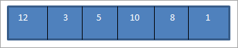
Այժմ յուրաքանչյուր անցման համար մենք ընթացիկ տարրը համեմատում ենք նրա բոլոր նախորդ տարրերի հետ: Այսպիսով, առաջին անցումում մենք սկսում ենք երկրորդ տարրից:
Այսպիսով, մենք պահանջում ենք N թվով անցումներ՝ N թվով տարրեր պարունակող զանգվածն ամբողջությամբ տեսակավորելու համար:
Վերոնշյալ նկարազարդումը կարելի է ամփոփել աղյուսակային տեսքով.
| Անցում | Չտեսակավորված ցուցակ | համեմատություն | Տեսակավորվածցուցակ |
|---|---|---|---|
| 1 | {12,3,5,10,8,1} | {12,3} | {3,12,5,10,8,1} |
| 2 | {3,12,5,10,8,1} | {3,12,5} | {3,5,12,10,8,1} |
| 3 | { 3,5,12,10,8,1} | {3,5,12,10} | {3,5,10,12,8,1} |
| 4 | {3,5,10,12,8,1} | {3,5,10,12,8} | {3,5,8,10,12,1} |
| 5 | {3,5,8,10,12,1} | {3,5,8,10,12,1} | {1,3,5,8,10,12} |
| 6 | {} | {} | {1,3,5,8,10,12} |
Ինչպես ցույց է տրված վերը նշված նկարում, մենք սկսում ենք 2-րդ տարրից, քանի որ ենթադրում ենք, որ առաջին տարրը միշտ տեսակավորված է: Այսպիսով, մենք սկսում ենք համեմատելով երկրորդ տարրը առաջինի հետ և փոխում ենք դիրքը, եթե երկրորդ տարրը փոքր է առաջինից: Այնուհետև մենք համեմատում ենք երրորդ տարրը նրա նախորդ (առաջին և երկրորդ) տարրերի հետ և կատարում ենք նույն ընթացակարգը՝ երրորդ տարրը ճիշտ տեղում տեղադրելու համար:
Այս կերպ, յուրաքանչյուր անցման համար մենք տեղադրում ենք մեկ տարր իր տեղը։ Առաջին անցման համար մենք տեղադրում ենք երկրորդ տարրը իր տեղում: Այսպիսով, ընդհանուր առմամբ, N տարրերն իրենց ճիշտ տեղում տեղադրելու համար մեզ անհրաժեշտ են N-1 անցումներ:
Հաջորդում մենք կցուցադրենք Insertion sort տեխնիկայի իրականացումը C++ լեզվով:
C++ Օրինակ
#include using namespace std; int main () { int myarray[10] = { 12,4,3,1,15,45,33,21,10,2}; cout"\nInput list is \n"; for(int i=0;i10;i++) { cout ="" Output:
Input list is
12 4 3 1 15 45 33 21 10 2
Sorted list is
1 2 3 4 10 12 15 21 33 45
Next, we will see the Java implementation of the Insertion sort technique.
Java Example
public class Main { public static void main(String[] args) { int[] myarray = {12,4,3,1,15,45,33,21,10,2}; System.out.println("Input list of elements ..."); for(int i=0;i10;i++) { System.out.print(myarray[i] + " "); } for(int k=1; k=0 && temp = myarray[j]) { myarray[j+1] = myarray[j]; j = j-1; } myarray[j+1] = temp; } System.out.println("\nsorted list of elements ..."); for(int i=0;i10;i++) { System.out.print(myarray[i] + " "); } } } Output:
Input list of elements …
12 4 3 1 15 45 33 21 10 2
sorted list of elements …
1 2 3 4 10 12 15 21 33 45
In both the implementations, we can see that we begin sorting from the 2nd element of the array (loop variable j = 1) and repeatedly compare the current element to all its previous elements and then sort the element to place it in its correct position if the current element is not in order with all its previous elements.
Insertion sort works the best and can be completed in fewer passes if the array is partially sorted. But as the list grows bigger, its performance decreases. Another advantage of Insertion sort is that it is a Stable sort which means it maintains the order of equal elements in the list.
Complexity Analysis Of The Insertion Sort Algorithm
From the pseudo code and the illustration above, insertion sort is the efficient algorithm when compared to bubble sort or selection sort. Instead of using for loop and present conditions, it uses a while loop that does not perform any more extra steps when the array is sorted.
However, even if we pass the sorted array to the Insertion sort technique, it will still execute the outer for loop thereby requiring n number of steps to sort an already sorted array. This makes the best time complexity of insertion sort a linear function of N where N is the number of elements in the array.
Thus the various complexities for Insertion sort technique are given below:
Worst case time complexity O(n 2 ) Best case time complexity O(n) Average time complexity O(n 2 ) Space complexity O(1)
In spite of these complexities, we can still conclude that Insertion sort is the most efficient algorithm when compared with the other sorting techniques like Bubble sort and Selection sort.
Conclusion
Insertion sort is the most efficient of all the three techniques discussed so far. Here, we assume that the first element is sorted and then repeatedly compare every element to all its previous elements and then place the current element in its correct position in the array.
In this tutorial, while discussing Insertion sort we have noticed that we compare the elements using an increment of 1 and also they are contiguous. This feature results in requiring more passes to get the sorted list.
In our upcoming tutorial, we will discuss “Shell sort” which is an improvement over the Selection sort.
In shell sort, we introduce a variable known as “increment” or a “gap” using which we divide the list into sublists containing non-contiguous elements that “gap” apart. Shell sort requires fewer passes when compared to Insertion sort and is also faster.
In our future tutorials, we will learn about two sorting techniques, “Quicksort” and “Mergesort” which use “Divide and conquer” strategy for sorting data lists.