- Агляд
- Агульны алгарытм
- Псеўдакод
- Ілюстрацыя
- Прыклад C++
- Java Example
- Complexity Analysis Of The Insertion Sort Algorithm
- Conclusion
Глыбокі погляд на сартаванне ўстаўкай з класічнымі прыкладамі.
Сартаванне ўстаўкай - гэта метад сартавання, які можна разглядаць так, як мы гуляем у карты. Тое, як мы ўстаўляем любую карту ў калоду або выдаляем яе, сартаванне ўстаўкай працуе падобным чынам.
Тэхніка алгарытму сартавання ўстаўкай больш эфектыўная, чым метады сартавання бурбалкай і выбарам, але менш эфектыўныя, чым іншыя метады напрыклад Quicksort і Merge sort.

Агляд
У тэхніцы сартавання ўстаўкай мы пачынаем з другога элемента, параўноўваем яго з першым элементам і змяшчаем у належным месцы. Затым мы выконваем гэты працэс для наступных элементаў.
Мы параўноўваем кожны элемент з усімі яго папярэднімі элементамі і змяшчаем або ўстаўляем элемент у патрэбнае месца. Тэхніка сартавання ўстаўкай больш прыдатная для масіваў з меншай колькасцю элементаў. Гэта таксама карысна для сартаваньня зьвязаных сьпісаў.
Звязаныя сьпісы маюць паказальнік на наступны элемэнт (у выпадку адно зьвязанага сьпісу) і таксама паказальнік на папярэдні элемэнт (у выпадку дзьвюхзьвязанага сьпісу ). Такім чынам, становіцца лягчэй рэалізаваць сартаванне ўстаўкай для звязанага спісу.
Давайце вывучым усё пра сартаванне ўстаўкай у гэтым уроку.
Агульны алгарытм
Крок 1 : Паўтарыце крокі з 2 па 5 для K = 1 да N-1
Крок 2 : усталюйце тэмпературу = A[K]
Крок 3 : усталюйце J = K– 1
Крок 4 : Паўтарыце, пакуль тэмпература =A[J]
усталявана A[J + 1] = A[J]
усталяваць J = J – 1
[канец унутранага цыклу]
Крок 5 : усталяваць A[J + 1] = тэмп
[ канец цыкла]
Крок 6 : выхад
Такім чынам, у тэхніцы сартавання ўстаўкай мы пачынаем з другога элемента, паколькі мяркуем, што першы элемент заўсёды адсартаваны . Затым ад другога элемента да апошняга мы параўноўваем кожны элемент з усімі яго папярэднімі элементамі і змяшчаем гэты элемент у патрэбнае месца.
Псеўдакод
Псеўдакод для сартаванне ўстаўкай прыведзена ніжэй.
procedure insertionSort(array,N ) array – array to be sorted N- number of elements begin int freePosition int insert_val for i = 1 to N -1 do: insert_val = array[i] freePosition = i //locate free position to insert the element whilefreePosition> 0 and array[freePosition -1] >insert_val do: array [freePosition] = array [freePosition -1] freePosition = freePosition -1 end while //insert the number at free position array [freePosition] = insert_val end for end procedure
Вышэй прыведзены псеўдакод для сартавання ўстаўкай, далей мы праілюструем гэтую тэхніку ў наступным прыкладзе.
Ілюстрацыя
Масіў для сартавання выглядае наступным чынам:
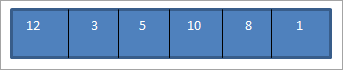
Цяпер для кожнага праходу мы параўноўваем бягучы элемент з усімі яго папярэднімі элементамі. Такім чынам, у першым праходзе мы пачынаем з другога элемента.
Такім чынам, нам патрабуецца N праходаў, каб цалкам адсартаваць масіў, які змяшчае N элементаў.
Вышэйпрыведзеная ілюстрацыя можа быць абагулена ў выглядзе табліцы:
| Прайшла | Неадсартаваны спіс | параўнанне | Адсартаванаспіс |
|---|---|---|---|
| 1 | {12,3,5,10,8,1} | {12,3} | {3,12,5,10,8,1} |
| 2 | {3,12,5,10,8,1} | {3,12,5} | {3,5,12,10,8,1} |
| 3 | { 3,5,12,10,8,1} | {3,5,12,10} | {3,5,10,12,8,1} |
| 4 | {3,5,10,12,8,1} | {3,5,10,12,8} | {3,5,8,10,12,1} |
| 5 | {3,5,8,10,12,1} | {3,5,8,10,12,1} | {1,3,5,8,10,12} |
| 6 | {} | {} | {1,3,5,8,10,12} |
Як паказана ў на ілюстрацыі вышэй, мы пачынаем з 2-га элемента, паколькі мяркуем, што першы элемент заўсёды адсартаваны. Такім чынам, мы пачынаем з параўнання другога элемента з першым і мяняем месца, калі другі элемент меншы за першы.
Гэты працэс параўнання і замены месцамі размяшчае два элементы на належных месцах. Затым мы параўноўваем трэці элемент з яго папярэднімі (першым і другім) элементамі і выконваем тую ж працэдуру, каб размясціць трэці элемент у належным месцы.
Такім чынам, для кожнага праходу мы змяшчаем адзін элемент у сваё месца. Для першага праходу на яго месца змяшчаем другі элемент. Такім чынам, увогуле, каб размясціць N элементаў у належным месцы, нам спатрэбіцца N-1 праходаў.
Далей мы прадэманструем рэалізацыю тэхнікі сартавання ўстаўкай на мове C++.
Прыклад C++
#include using namespace std; int main () { int myarray[10] = { 12,4,3,1,15,45,33,21,10,2}; cout"\nInput list is \n"; for(int i=0;i10;i++) { cout ="" Output:
Input list is
12 4 3 1 15 45 33 21 10 2
Sorted list is
1 2 3 4 10 12 15 21 33 45
Next, we will see the Java implementation of the Insertion sort technique.
Java Example
public class Main { public static void main(String[] args) { int[] myarray = {12,4,3,1,15,45,33,21,10,2}; System.out.println("Input list of elements ..."); for(int i=0;i10;i++) { System.out.print(myarray[i] + " "); } for(int k=1; k=0 && temp = myarray[j]) { myarray[j+1] = myarray[j]; j = j-1; } myarray[j+1] = temp; } System.out.println("\nsorted list of elements ..."); for(int i=0;i10;i++) { System.out.print(myarray[i] + " "); } } } Output:
Input list of elements …
12 4 3 1 15 45 33 21 10 2
sorted list of elements …
1 2 3 4 10 12 15 21 33 45
In both the implementations, we can see that we begin sorting from the 2nd element of the array (loop variable j = 1) and repeatedly compare the current element to all its previous elements and then sort the element to place it in its correct position if the current element is not in order with all its previous elements.
Insertion sort works the best and can be completed in fewer passes if the array is partially sorted. But as the list grows bigger, its performance decreases. Another advantage of Insertion sort is that it is a Stable sort which means it maintains the order of equal elements in the list.
Complexity Analysis Of The Insertion Sort Algorithm
From the pseudo code and the illustration above, insertion sort is the efficient algorithm when compared to bubble sort or selection sort. Instead of using for loop and present conditions, it uses a while loop that does not perform any more extra steps when the array is sorted.
However, even if we pass the sorted array to the Insertion sort technique, it will still execute the outer for loop thereby requiring n number of steps to sort an already sorted array. This makes the best time complexity of insertion sort a linear function of N where N is the number of elements in the array.
Thus the various complexities for Insertion sort technique are given below:
Worst case time complexity O(n 2 ) Best case time complexity O(n) Average time complexity O(n 2 ) Space complexity O(1)
In spite of these complexities, we can still conclude that Insertion sort is the most efficient algorithm when compared with the other sorting techniques like Bubble sort and Selection sort.
Conclusion
Insertion sort is the most efficient of all the three techniques discussed so far. Here, we assume that the first element is sorted and then repeatedly compare every element to all its previous elements and then place the current element in its correct position in the array.
In this tutorial, while discussing Insertion sort we have noticed that we compare the elements using an increment of 1 and also they are contiguous. This feature results in requiring more passes to get the sorted list.
In our upcoming tutorial, we will discuss “Shell sort” which is an improvement over the Selection sort.
In shell sort, we introduce a variable known as “increment” or a “gap” using which we divide the list into sublists containing non-contiguous elements that “gap” apart. Shell sort requires fewer passes when compared to Insertion sort and is also faster.
In our future tutorials, we will learn about two sorting techniques, “Quicksort” and “Mergesort” which use “Divide and conquer” strategy for sorting data lists.