- Baxış
- Ümumi alqoritm
- Pseudocode
- İllüstrasiya
- C++ Misal
- Java Example
- Complexity Analysis Of The Insertion Sort Algorithm
- Conclusion
Klassik Nümunələrlə Daxiletmə Sortuna Dərindən Baxış.
Daxiletmə çeşidləmə əlimizdə kart oynayacağımız şəkildə baxıla bilən çeşidləmə texnikasıdır. İstənilən kartı göyərtəyə daxil etməyimiz və ya onu çıxarmağımız, daxil etmə çeşidləmələri oxşar şəkildə işləyir.
Daxiletmə çeşidləmə alqoritmi texnikası Bubble çeşidləmə və Seçmə çeşidləmə üsullarından daha səmərəlidir, lakin digər üsullardan daha az səmərəlidir. Quicksort və Merge sort kimi.

Baxış
Daxiletmə çeşidləmə texnikasında biz ikinci elementdən başlayırıq və onu birinci elementlə müqayisə edirik və onu qoyuruq. lazımi yerdə. Sonra biz bu prosesi sonrakı elementlər üçün yerinə yetiririk.
Hər bir elementi bütün əvvəlki elementləri ilə müqayisə edirik və elementi öz uyğun yerinə qoyuruq və ya daxil edirik. Daxiletmə çeşidləmə texnikası daha az sayda elementə malik massivlər üçün daha məqsədəuyğundur. O, həmçinin əlaqəli siyahıları çeşidləmək üçün faydalıdır.
Əlaqəli siyahılarda növbəti elementə (tək bağlı siyahı olduqda) və əvvəlki elementə də (ikiqat əlaqəli siyahı olduqda) göstərici var. ). Beləliklə, əlaqəli siyahı üçün daxiletmə növünü həyata keçirmək daha asan olur.
Gəlin bu dərslikdə Daxiletmə çeşidi haqqında hər şeyi araşdıraq.
Ümumi alqoritm
Addım 1 : K = 1 - N-1
Addım 2 : temp = A[K] üçün 2-dən 5-ə qədər addımları təkrarlayın
Addım 3 : J = K təyin edin– 1
Addım 4 : Temp =A[J]
A[J + 1] = A[J]
0 təyin edərkən təkrarlayın>dəst J = J – 1[daxili döngənin sonu]
Addım 5 : təyin A[J + 1] = temp
[ loopun sonu]
Addım 6 : exit
Beləliklə, daxil etmə çeşidləmə texnikasında birinci elementin həmişə çeşidləndiyini fərz etdiyimiz üçün ikinci elementdən başlayırıq. . Sonra ikinci elementdən sonuncu elementə qədər hər bir elementi onun bütün əvvəlki elementləri ilə müqayisə edirik və həmin elementi lazımi yerə qoyuruq.
Pseudocode
Pseudo-kod daxiletmə çeşidi aşağıda verilmişdir.
procedure insertionSort(array,N ) array – array to be sorted N- number of elements begin int freePosition int insert_val for i = 1 to N -1 do: insert_val = array[i] freePosition = i //locate free position to insert the element whilefreePosition> 0 and array[freePosition -1] >insert_val do: array [freePosition] = array [freePosition -1] freePosition = freePosition -1 end while //insert the number at free position array [freePosition] = insert_val end for end procedure
Yuxarıda Daxiletmə çeşidi üçün psevdokod verilmişdir, bundan sonra biz bu texnikanı aşağıdakı nümunədə təsvir edəcəyik.
İllüstrasiya
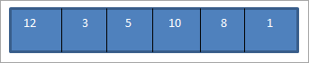
Normallaşdırılacaq massiv aşağıdakı kimidir:
İndi hər keçid üçün cari elementi onun bütün əvvəlki elementləri ilə müqayisə edirik. Beləliklə, birinci keçiddə biz ikinci elementdən başlayırıq.
Beləliklə, N sayda elementdən ibarət massivi tamamilə çeşidləmək üçün N sayda keçid tələb olunur.
Yuxarıdakı illüstrasiya cədvəl şəklində ümumiləşdirilə bilər:
| Keçid | Çeşidlənməmiş siyahı | müqayisə | Sıralandısiyahı |
|---|---|---|---|
| 1 | {12,3,5,10,8,1} | {12,3} | {3,12,5,10,8,1} |
| 2 | {3,12,5,10,8,1} | {3,12,5} | {3,5,12,10,8,1} |
| 3 | { 3,5,12,10,8,1} | {3,5,12,10} | {3,5,10,12,8,1} |
| 4 | {3,5,10,12,8,1} | {3,5,10,12,8} | {3,5,8,10,12,1} |
| 5 | {3,5,8,10,12,1} | {3,5,8,10,12,1} | {1,3,5,8,10,12} |
| 6 | {} | {} | {1,3,5,8,10,12} |
Göstərildiyi kimi yuxarıdakı təsvirdə, birinci elementin həmişə çeşidləndiyini güman etdiyimiz üçün 2-ci elementdən başlayırıq. Beləliklə, biz ikinci elementi birinci ilə müqayisə etməklə başlayırıq və əgər ikinci element birincidən kiçikdirsə, mövqeyi dəyişdiririk.
Bu müqayisə və dəyişdirmə prosesi iki elementi öz uyğun yerlərində yerləşdirir. Sonra üçüncü elementi əvvəlki (birinci və ikinci) elementləri ilə müqayisə edirik və üçüncü elementi lazımi yerə yerləşdirmək üçün eyni proseduru yerinə yetiririk.
Beləliklə, hər keçid üçün bir element yerləşdiririk. onun yeri. Birinci keçid üçün ikinci elementi öz yerinə qoyuruq. Beləliklə, ümumiyyətlə, N elementi öz yerində yerləşdirmək üçün bizə N-1 keçid lazımdır.
Sonra biz C++ dilində Insertion sort texnikasının həyata keçirilməsini nümayiş etdirəcəyik.
C++ Misal
#include using namespace std; int main () { int myarray[10] = { 12,4,3,1,15,45,33,21,10,2}; cout"\nInput list is \n"; for(int i=0;i10;i++) { cout ="" Output:
Input list is
12 4 3 1 15 45 33 21 10 2
Sorted list is
1 2 3 4 10 12 15 21 33 45
Next, we will see the Java implementation of the Insertion sort technique.
Java Example
public class Main { public static void main(String[] args) { int[] myarray = {12,4,3,1,15,45,33,21,10,2}; System.out.println("Input list of elements ..."); for(int i=0;i10;i++) { System.out.print(myarray[i] + " "); } for(int k=1; k=0 && temp = myarray[j]) { myarray[j+1] = myarray[j]; j = j-1; } myarray[j+1] = temp; } System.out.println("\nsorted list of elements ..."); for(int i=0;i10;i++) { System.out.print(myarray[i] + " "); } } } Output:
Input list of elements …
12 4 3 1 15 45 33 21 10 2
sorted list of elements …
1 2 3 4 10 12 15 21 33 45
In both the implementations, we can see that we begin sorting from the 2nd element of the array (loop variable j = 1) and repeatedly compare the current element to all its previous elements and then sort the element to place it in its correct position if the current element is not in order with all its previous elements.
Insertion sort works the best and can be completed in fewer passes if the array is partially sorted. But as the list grows bigger, its performance decreases. Another advantage of Insertion sort is that it is a Stable sort which means it maintains the order of equal elements in the list.
Complexity Analysis Of The Insertion Sort Algorithm
From the pseudo code and the illustration above, insertion sort is the efficient algorithm when compared to bubble sort or selection sort. Instead of using for loop and present conditions, it uses a while loop that does not perform any more extra steps when the array is sorted.
However, even if we pass the sorted array to the Insertion sort technique, it will still execute the outer for loop thereby requiring n number of steps to sort an already sorted array. This makes the best time complexity of insertion sort a linear function of N where N is the number of elements in the array.
Thus the various complexities for Insertion sort technique are given below:
Worst case time complexity O(n 2 ) Best case time complexity O(n) Average time complexity O(n 2 ) Space complexity O(1)
In spite of these complexities, we can still conclude that Insertion sort is the most efficient algorithm when compared with the other sorting techniques like Bubble sort and Selection sort.
Conclusion
Insertion sort is the most efficient of all the three techniques discussed so far. Here, we assume that the first element is sorted and then repeatedly compare every element to all its previous elements and then place the current element in its correct position in the array.
In this tutorial, while discussing Insertion sort we have noticed that we compare the elements using an increment of 1 and also they are contiguous. This feature results in requiring more passes to get the sorted list.
In our upcoming tutorial, we will discuss “Shell sort” which is an improvement over the Selection sort.
In shell sort, we introduce a variable known as “increment” or a “gap” using which we divide the list into sublists containing non-contiguous elements that “gap” apart. Shell sort requires fewer passes when compared to Insertion sort and is also faster.
In our future tutorials, we will learn about two sorting techniques, “Quicksort” and “Mergesort” which use “Divide and conquer” strategy for sorting data lists.